写在前面的话

本文主要是基于Pytorch给出的官方Tutorial，然后我按照自己的喜好编辑成Jupyter文档，后转成本博客，用来作为自己的日常参照材料。

Pytorch

Pytorch给我的感觉是：它是基于更高级的封装，实现深度学习更加简单，比较适合科研型的或者是实现一些想法的入门级选手。Tensorflow更适合工程项目，能够比较高效的运行。但是对于一般选手来说，Pytorch更适合，因为它是动态图，在个人代码水平不是很高的情况下，Pytorch的效率是高于Tensorflow的。

1
2
3

from __future__ import print_function
import torch
device = torch.device( "cuda" if torch.cuda.is_available() else "cpu")

Tensors

# Contruct a 2x1 matric, uninitialized:
x = torch.empty(2, 1, device=device)
print(x)

tensor([[0.0000],
        [0.0000]])

1
2
3

# Construct a randomly initialized matrix:
x = torch.rand(5, 3, device=device)
print(x)

tensor([[0.2854, 0.5359, 0.7811],
        [0.1065, 0.0246, 0.3945],
        [0.8341, 0.6808, 0.4578],
        [0.4257, 0.7255, 0.3597],
        [0.3510, 0.3170, 0.1526]])

1
2
3

# Construct a matrix filled zeros and dtype long
x = torch.zeros(2, 1, dtype=torch.long, device=device)
print(x)

tensor([[0],
        [0]])

1
2
3

# Construct a tensor directly from data;
x = torch.tensor([3, 3])
print(x)

tensor([3, 3])

x = x.new_ones(2, 1, dtype=torch.double) # new_* methods take in size
print(x)

x = torch.randn_like(x, dtype=torch.float) # override dype and result has same size
print(x)

tensor([[1.],
        [1.]], dtype=torch.float64)
tensor([[1.4535],
        [0.0968]])

# get its size
print(x.size())

print(x.shape)

torch.Size([2, 1])
torch.Size([2, 1])

Opertions

# Addition
x = x.new_ones(3, 2, dtype=torch.float)
y = torch.rand(3, 2, dtype=torch.float)
print(x + y) # syntax 1
print(torch.add(x, y)) # syntax 2
result = torch.empty(5, 6)
torch.add(x, y, out=result) # add x and y to result
print(result)
y.add_(x)
print(y) # add x to y

tensor([[1.9447, 1.9085],
        [1.3177, 1.8074],
        [1.1208, 1.8663]])
tensor([[1.9447, 1.9085],
        [1.3177, 1.8074],
        [1.1208, 1.8663]])
tensor([[1.9447, 1.9085],
        [1.3177, 1.8074],
        [1.1208, 1.8663]])
tensor([[1.9447, 1.9085],
        [1.3177, 1.8074],
        [1.1208, 1.8663]])

注：任何tensor后面带有下划线都会改变tensor的值，比如x.copy_(y), x.t_(x)

1
2
3

x = torch.rand(3, 2)
print(x)
print(x[:, 1])

tensor([[0.8368, 0.9204],
        [0.3797, 0.0908],
        [0.4454, 0.7684]])
tensor([0.9204, 0.0908, 0.7684])

# resizing
x = torch.randn(4, 4)
y = x.view(16)
z = x.view(-1, 8) # the size -1 is inferred from other dimensions
print(x.size(), y.size(), z.size())

torch.Size([4, 4]) torch.Size([16]) torch.Size([2, 8])

# Converting Numpy Array to Torch Tensor
import numpy as np
a = np.ones(5)
b = torch.from_numpy(a)
np.add(a, 1, out=a)
print(a)
print(b)

[2. 2. 2. 2. 2.]
tensor([2., 2., 2., 2., 2.], dtype=torch.float64)

# CUDA Tensor
if torch.cuda.is_available():
    device = torch.device("cuda")
    y = torch.ones_like(x, device=device)
    x = x.to(device)
    z = x + y
    print(z)
    print(z.to("cpu", torch.double))

Define the Network

1
2
3

import torch
import torch.nn as nn
import torch.nn.functional as F

本来这个网络应该是LeNet的，输入要求是32x32，我改变了第一个全连接层，将输入变为了20x20。
所以网络结构可以通过自己的想法进行改变，最重要的是改变全连接层就可以了。
网络经过卷积之后输入的结果公式为：$$ outputsize = （inputsize - kernelsize + 2 * pad）/stride + 1 $$

class Net(nn.Module):

    def __init__(self):
        super(Net, self).__init__()
        # 1 input image channel, 6 output channels, 5x5 square convolution
        # kernel
        self.conv1 = nn.Conv2d(1, 6, 5)
        self.conv2 = nn.Conv2d(6, 16, 5)
        # an affine operation: y = Wx + b
        self.fc1 = nn.Linear(16 * 2 * 2, 120)
        self.fc2 = nn.Linear(120, 84)
        self.fc3 = nn.Linear(84, 10)
        
    def forward(self, x):
        # Max pooling over a (2, 2) window
        x = F.max_pool2d(F.relu(self.conv1(x)), (2, 2))
        # if the size is a square you can only specify a single number 
        x = F.max_pool2d(F.relu(self.conv2(x)), 2)
        x = x.view(-1, self.num_flat_feature(x))
        x = F.relu(self.fc1(x))
        x = F.relu(self.fc2(x))
        x = F.relu(self.fc3(x))
        return x
    
    def num_flat_feature(self, x):
        size = x.size()[1:] # all dimensions except the batch dimension
        num_features = 1
        for s in size:
            num_features *= s 
        return num_features
net = Net()
print(net)

Net(
  (conv1): Conv2d(1, 6, kernel_size=(5, 5), stride=(1, 1))
  (conv2): Conv2d(6, 16, kernel_size=(5, 5), stride=(1, 1))
  (fc1): Linear(in_features=64, out_features=120, bias=True)
  (fc2): Linear(in_features=120, out_features=84, bias=True)
  (fc3): Linear(in_features=84, out_features=10, bias=True)
)

# The learnable parameter of a model are returned by net.parameters()
params = list(net.parameters())
print(len(params))
print(params[0].size()) # conv1's .weights

10
torch.Size([6, 1, 5, 5])

1
2
3

input = torch.randn(1, 1, 20, 20)
out = net(input)
print(out)

tensor([[0.0432, 0.1072, 0.0000, 0.1096, 0.0378, 0.0000, 0.0000, 0.0000, 0.0202,
         0.0000]], grad_fn=<ReluBackward>)

zero the gradients

1 2	net.zero_grad() out.backward(torch.randn(1, 10))

torch.nn only supports mini-batches. The entire torch.nn package only supports inputs that are a mini-batch of samples, and not a single sample.
For example, nn.Conv2d will take in a 4D Tensor of nSamples x nChannels x Height x Width.
If you have a single sample, just use input.unsqueeze(0) to add a fake batch dimension.

Loss Function

out = net(input)
target = torch.randn(10) # a dummy target, for example 
target = target.view(1, -1)
criterion = nn.MSELoss()

loss = criterion(out, target)
print(loss)

tensor(1.7536, grad_fn=<MseLossBackward>)

forward:
input -> conv2d -> relu -> maxpool2d -> conv2d -> relu -> maxpool2d
-> view -> linear -> relu -> linear -> relu -> linear
-> MSELoss
-> loss

1
2
3

print(loss.grad_fn) # MSELoss
print(loss.grad_fn.next_functions[0][0]) # Linear
print(loss.grad_fn.next_functions[0][0].next_functions[0][0]) # relu

<MseLossBackward object at 0x0000000008619780>
<ReluBackward object at 0x0000000008619A58>
<ThAddmmBackward object at 0x0000000008619780>

Backpropagate

net.zero_grad() # zeros the gradient buffer of all parameters 
print('conv1.bias.grad before backward')
print(net.conv1.bias.grad)

# loss.backward() # 为了和下面的产生两次相同的backpropagate，所以将这里注释，下一个单元也是这样。

print('conv1.bias.grad before backward')
print(net.conv1.bias.grad)

conv1.bias.grad before backward
tensor([0., 0., 0., 0., 0., 0.])
conv1.bias.grad before backward
tensor([0., 0., 0., 0., 0., 0.])

## Weights
# learning_rate = 0.01
# for f in net.parameters():
#     f.data.sub_(f.grad.data * learning_rate)  # f = f - learning_rate * gradient

import torch.optim as optim

# creater your optimizer
optimizer = optim.SGD(net.parameters(), lr=0.01)

# in your training loop 
optimizer.zero_grad() # zero the gradient buffers
output = net(input)
loss = criterion(out, target)
loss.backward()
optimizer.step() # Does the update

Training A Classifier

1
2
3

import torch
import torchvision
import torchvision.transforms as transforms

# The output of torchvision datasets are PILImage iamges of range [0, 1]. We transform them to Tensor of normalized range [-1, 1]
transform = transforms.Compose(
[transforms.ToTensor(), transforms.Normalize((0.5, 0.5, 0.5), (0.5, 0.5, 0.5))])

trainset = torchvision.datasets.CIFAR10(root='./data', train=True, 
                                       download=True, transform=transform)
trainloader = torch.utils.data.DataLoader(trainset, batch_size=4, 
                                          shuffle=True, num_workers=2)

testset = torchvision.datasets.CIFAR10(root='./data', train=False, 
                                      download=True, transform=transform)
testloader = torch.utils.data.DataLoader(testset, batch_size=4, 
                                              shuffle=False, num_workers=2)
classes = ('plane', 'car', 'bird', 'cat', 
          'deer', 'dog', 'frog', 'horse', 'ship', 'truck')

Files already downloaded and verified
Files already downloaded and verified

import matplotlib.pyplot as plt 
import numpy as np

def imshow(img):
    img = img/2 + 0.5 # unnormalize
    npimg = img.numpy()
#     print(npimg.shape)
    plt.imshow(np.transpose(npimg, (1, 2, 0)))
#     print(np.transpose(npimg, (1, 2, 0)).shape)
    
# get some random training images
dataiter = iter(trainloader)
images, labels = dataiter.next()
# print(labels)
# show images
imshow(torchvision.utils.make_grid(images)) # 制作图像网格
plt.show()
# print labels
print(' '.join('%5s' % classes[labels[j]] for j in range(4)))

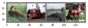
 deer truck plane horse

Define a Convolution Neural Network

import torch.nn as nn
import torch.nn.functional as F

class Net(nn.Module):
    def __init__(self):
        super(Net, self).__init__()
        self.conv1 = nn.Conv2d(3, 6, 5)
        self.pool = nn.MaxPool2d(2, 2)
        self.conv2 = nn.Conv2d(6, 16, 5)
        self.fc1 = nn.Linear(16 * 5 * 5, 120)
        self.fc2 = nn.Linear(120, 84)
        self.fc3 = nn.Linear(84, 10)
    def forward(self, x):
        x = self.pool(F.relu(self.conv1(x)))
        x = self.pool(F.relu(self.conv2(x)))
        x = x.view(-1, 16 * 5 * 5)
        x = F.relu(self.fc1(x))
        x = F.relu(self.fc2(x))
        x = self.fc3(x)
        return x

net = Net()
net.to(device)
print(net)

Net(
  (conv1): Conv2d(3, 6, kernel_size=(5, 5), stride=(1, 1))
  (pool): MaxPool2d(kernel_size=2, stride=2, padding=0, dilation=1, ceil_mode=False)
  (conv2): Conv2d(6, 16, kernel_size=(5, 5), stride=(1, 1))
  (fc1): Linear(in_features=400, out_features=120, bias=True)
  (fc2): Linear(in_features=120, out_features=84, bias=True)
  (fc3): Linear(in_features=84, out_features=10, bias=True)
)

Define a Loss function and opotimizer

import  torch.optim as optim

criterion = nn.CrossEntropyLoss()
optimizer = optim.SGD(net.parameters(), lr=0.001, momentum=0.9)

Train the network

for epoch in range(2):
    running_loss = 0.0
    for i, data in enumerate(trainloader, 0):
        # get the inputs 
        inputs, labels = data 
        inputs, labels = inputs.to(device), labels.to(device)
        # zero the parameter gradients
        optimizer.zero_grad()
        
        # forward  + backward + optimize
        outputs = net(inputs)
        loss = criterion(outputs, labels)
        loss.backward()
        optimizer.step()
        
        # print statistics
        running_loss += loss.item()
        if i % 2000 == 1999: # print every 2000 mini-batches 
            print('[%d, %5d] loss: %.3f' % 
                 (epoch + 1, i + 1, running_loss / 2000))
            running_loss = 0.0
print('Finished Training')

[1,  2000] loss: 2.217
[1,  4000] loss: 1.855
[1,  6000] loss: 1.672
[1,  8000] loss: 1.570
[1, 10000] loss: 1.506
[1, 12000] loss: 1.461
[2,  2000] loss: 1.370
[2,  4000] loss: 1.369
[2,  6000] loss: 1.340
[2,  8000] loss: 1.323
[2, 10000] loss: 1.276
[2, 12000] loss: 1.279
Finished Training

dataiter = iter(testloader)
images, labels = dataiter.next()

# print images 
imshow(torchvision.utils.make_grid(images))
plt.show()
print('GroundTruth: ', ' '.join('%5s' % classes[labels[j]] for j in range(4)))

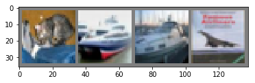
GroundTruth:    cat  ship  ship plane

1 2	outputs = net(images) print(outputs)

tensor([[-0.7807, -1.7329,  0.9516,  1.8043, -1.2077,  0.7349,  1.3615, -1.5412,
          1.0311, -1.7234],
        [ 5.2413,  6.1315, -1.7400, -3.2287, -5.0497, -5.8038, -4.2375, -4.4465,
          7.7529,  4.1842],
        [ 2.7686,  3.8909, -0.7050, -1.7185, -3.2625, -3.2960, -2.2888, -2.6324,
          3.8761,  2.4697],
        [ 4.0929,  1.8480,  0.1962, -1.7907, -1.6931, -3.4538, -2.2210, -3.0694,
          4.5059,  0.7960]], grad_fn=<ThAddmmBackward>)

1
2
3

_, predicted = torch.max(outputs, 1)
print(predicted)
print('Predicted: ', ' '.join('%5s' % classes[predicted[j]] for j in range(4)))

tensor([3, 8, 1, 8])
Predicted:    cat  ship   car  ship

correct = 0
total = 0
with torch.no_grad():
    for data in testloader:
        images, labels = data
#         print(labels)
        outputs = net(images)
        _, predicted = torch.max(outputs.data, 1)
        total += labels.size(0)
        correct += (predicted == labels).sum().item()

print('Accuracy of the network on the 10000 test images: %d %%' % (
    100 * correct / total))

Accuracy of the network on the 10000 test images: 54 %

class_correct = list(0. for i in range(10))
class_total = list(0. for i in range(10))
with torch.no_grad():
    for data in testloader:
        images, labels = data
        outputs = net(images)
        _, predicted = torch.max(outputs, 1) # torch.max 可以返回最大值和对应的坐标，np.random.randn只能返回最大值
        c = (predicted == labels).squeeze()
        for i in range(4):
            label = labels[i]
            class_correct[label] += c[i].item()
            class_total[label] += 1


for i in range(10):
    print('Accuracy of %5s : %2d %%' % (
        classes[i], 100 * class_correct[i] / class_total[i]))

Accuracy of plane : 55 %
Accuracy of   car : 59 %
Accuracy of  bird : 65 %
Accuracy of   cat : 29 %
Accuracy of  deer : 22 %
Accuracy of   dog : 49 %
Accuracy of  frog : 71 %
Accuracy of horse : 55 %
Accuracy of  ship : 75 %
Accuracy of truck : 62 %