写在前面的话
最近,十分困惑条件随机场是如何工作的,为什么可以加在卷积神经网络的后面作为后处理的部分。虽然理论部分前面的博客也有写过,做过一些总结,不过因为没有实现过代码,所以仍有困惑解决不了,每念至此,心绪不宁,遂作此文,以供参考。
具体实现
本文将实现全连接随机场对非RGB的图像进行分割,主要参考文献[1]以及对应的github代码,另外本文需要安装pydensecrf,可以通过pip install pydensecrf安装,安装时需注意,pydensecrf依赖于cython,需要先安装cython。
对非RGB图像分割
本文的代码放在了我的github中命名为CRF的仓库库中,链接地址,这里的代码来自于pydensecrf。
一元势
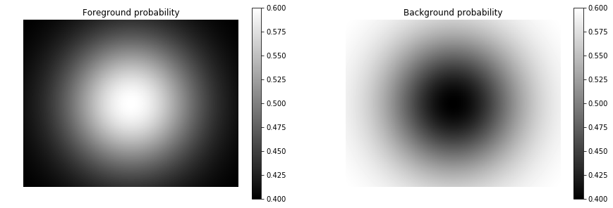
一元势包含了每个像素对应的类别,这些可以来自随机森林或者是深度神经网络的softmax。这里,我们共有两个类别,一个是前景,一个是背景,这里大小设置为$400\times 512$。我们建立了两个二维的高斯分布,并且平面显示。
1 | from scipy.stats import multivariate_normal |
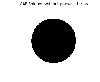
使用一元势进行推断
这里我们可以使用一元势进行推断,也就是说这里我们不考虑像素间的相互关联。这样做并不是很好的推断,但是可以这么做。
1 | # Inference without pair-wise terms |
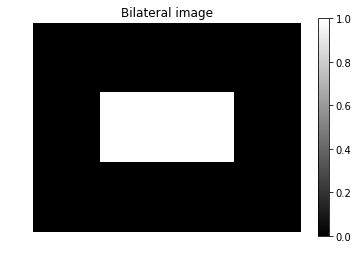
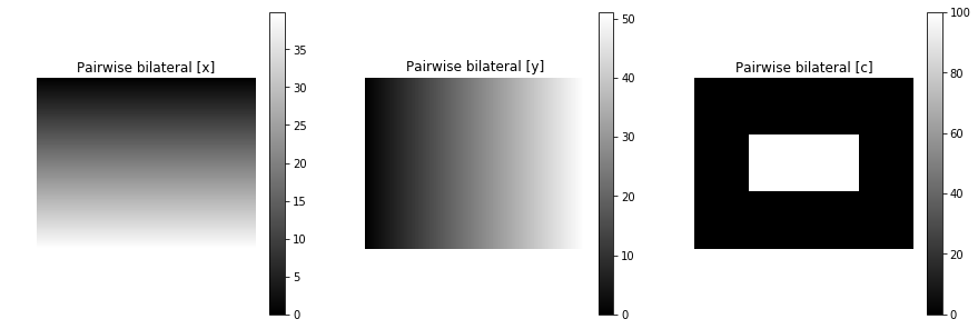
二元势
图像处理中,我们经常使用像素间的双边关系,也就是说,我们认为有相似颜色的或者是相似的位置的像素认为是同一类。下面我们建立这样的双边关系。
1 | NCHAN=1 |
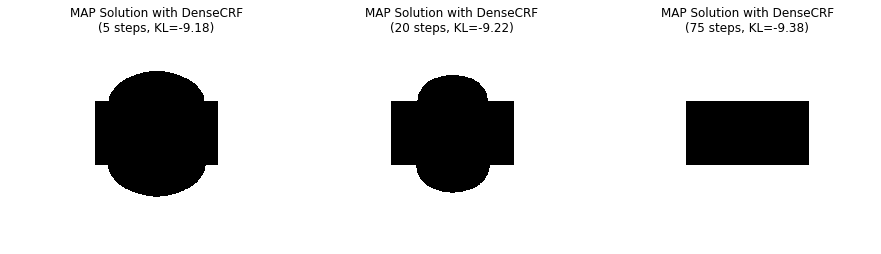
使用完整的条件随机场进行推断
下面我们将一元势与二元势结合起来进行推断,执行不同的迭代次数,有下面的结果。
1 | d = dcrf.DenseCRF2D(W, H, NLABELS) |
参考文献
[1] Krähenbühl P, Koltun V. Efficient inference in fully connected crfs with gaussian edge potentials[C]//Advances in neural information processing systems. 2011: 109-117.